Intro to fishflux
Nina M. D. Schiettekatte
2024-10-25
Source:vignettes/intro_to_fishflux.Rmd
intro_to_fishflux.RmdIntroduction
The fishflux package provides a tool to model fluxes of
C (carbon), N (nitrogen) and P (phosphorus) in fishes. It combines basic
principles from elemental stoichiometry and metabolic theory. The
package offers a user-friendly interface to apply the model.
fishflux is ideal for fish ecologists wishing to predict
ingestion, egestion and excretion to study fluxes of nutrients and
energy.
Main assets:
- Provides function to model fluxes of Carbon, Nitrogen and Phosphorus for fishes
- Allows for the estimation of uncertainty, dpending on the uncertainy of the input parameters
- Provides some functions to help find parameters as inputs for the model
- Provides functions to extract and illustrate results
Installing and loading fishflux
fishflux uses Markov Chain Monte Carlo simulations
provided by stan.
Therefore, the first step is to install rstan.
It’s important to closely follow all the steps described on the page
depending on your operating system.
Downloaded package file
Another option is to download the source file available on GitHub here.
install.packages(path_to_fishflux_file, repos = NULL, type = "source")How to use fishflux?
fishflux is designed to follow three simple steps:
- Find the right input parameters
- Run the model simulation with those input parameters
- Plot the model results and check sensitivity
Input parameters
Before running the model, the parameters have to be specified. Below,
there is a table showing all parameters needed to run the model
simulation. fishflux provides several functions to find
some of these parameters, but note that others have to be provided by
the user at this stage. Ideally, all parameters should also have a
standard deviation, so that their uncertainty can be reflected in the
model predictions
| Symbol | Description | Unit |
|---|---|---|
| ak | Element-specific assimilation efficiency | _ |
| lt | Total length of individual | cm |
| linf | Asymptotic adult length (VBGC) | cm |
| κ | Growth rate parameter (VBGC) | yr − 1 |
| t0 | Age at settlement (VBGC) | yr |
| lwa | Parameter length-weight relationship | g cm − 1 |
| lwb | Parameter length-weight relationship | _ |
| Qk | Element-specific body content percentage | % |
| f0 | Metabolic normalisation constant independent of body mass | g Cg − αd − 1 |
| alpha | Mass-scaling exponent | _ |
| theta | Activity scope | _ |
| v | Environmental temperature | C |
| h | trophic level | _ |
| r | Aspect ratio of caudal fin | _ |
| F0nz | Mass-specific turnover rate of N | g Ng − 1d − 1 |
| F0pz | Mass-specific turnover rate of P | g Pg − 1d − 1 |
| mdw | Ratio of dry mass and wet mass of fish | _ |
| Dk | Elemental stoichiometry of diet | % |
A good place to start is checking if you are using the correct
scientific name of your species of interest. The function
name_errors will tell you if the species name is correct.
This function can be useful, especially when working with larger
databases.
library(fishflux)
# example
name_errors("Zebrazoma scopas")
#> Joining with `by = join_by(Subfamily, GenCode, FamCode)`
#> Joining with `by = join_by(FamCode)`
#> Joining with `by = join_by(Order, Ordnum, Class, ClassNum)`
#> Joining with `by = join_by(Class, ClassNum)`
#> Inaccurate species names found:
#> [1] "Zebrazoma scopas"
Once the species names are verified and/or corrected we can continue with specifying some parameters.
The find_lw function searches FishBase to find length-weight
relationship parameters lw_a and lw_b
extracted from Froese and Pauly
(2018).
# example
find_lw("Zebrasoma scopas", mirror = "se")
#>            species   lwa_m      lwa_sd lwb_m    lwb_sd
#> 1 Zebrasoma scopas 0.02512 0.002709184  2.98 0.0255102
The model uses parameters von Bertalanffy’s growth model (VBGM) to
estimate growth rates. A quick way to get available information from
FishBase is the function growth_params(). This can be a
good indication, but users should interpret these estimates with a
critical eye, as they come from disparate sources of varying accuracy.
Alternatively, it is advised to use growth curves derived from otolith
readings. In the absence of otolith data, one might consider extracting
standardised estimations from Morais and Bellwood
(2018).
# example
# The option otolith=TRUE filters out sources that used otoliths for the estimation of growth parameters
growth_params("Sargocentron microstoma", otolith = FALSE)
#> # A tibble: 1 × 7
#>   species                 Locality                 k  Linf    t0 method comments
#>   <chr>                   <chr>                <dbl> <dbl> <dbl> <chr>  <chr>
#> 1 Sargocentron microstoma Tiahura reef, Moore…     1  18.6    NA lengt… NA
Further, there are a couple more basic functions to get an indication
of parameters that are available on FishBase such as
trophic_level() and aspect_ratio(). Note that
it is always better to get the approximations through analysis,
measurements and otolith analysis over parameters extracted from
functions, such as growth_params(),
trophic_level() and aspect_ratio(). To get an
overview of all parameters available, fishflux provides a
wrapper function model_parameters().
# example
zebsco <- model_parameters("Zebrasoma scopas", family = "Acanthuridae",
                           temp = 27, mirror = "se")
## Here we set the temperature at 27 degrees as an example, this the average sea temperature in Moorea, French Polynesia
print(zebsco)
#>            species    t0 Linf     k     asp troph   lwa_m      lwa_sd lwb_m
#> 1 Zebrasoma scopas -0.49 13.3 0.425 2.02091     2 0.02512 0.002709184  2.98
#>      lwb_sd     mdw_m        f0_m        f0_sd alpha_m   alpha_sd
#> 1 0.0255102 0.2504833 0.001517989 3.032338e-10    0.77 0.05286288
All other parameters have to be provided by the user. For more information on how to acquire these parameters, take a look at (“this paper” add reference to methods paper).
Run model
Once all the parameters are collected, we can run the model through
cnp_model_mcmc(). Note that this model can be run with or
without specifying the standard deviation (sd) of each parameter. If the
sd of a certain parameter is not provided, it will be automatically set
to a very low value (1-10). As mentioned before, it is
advisable to include uncertainty of parameters. fishflux is
designed to use the MCMC sampler in order to include uncertainty of
predictions.
## load the example parameters for Zebrasoma scopas, a list
data(param_zebsco)
## Run the model, specifying the target length(s) and the parameter list
model <- cnp_model_mcmc(TL = 5:20, param = param_zebsco)
#> Warning in FUN(X[[i]], ...): not inputting certain parameters may give wrong
#> results
#> Warning in FUN(X[[i]], ...): adding standard values for mdw_m
#> Warning in FUN(X[[i]], ...): adding standard values for lt_sd
#> Warning in FUN(X[[i]], ...): adding standard values for ac_sd
#> Warning in FUN(X[[i]], ...): adding standard values for an_sd
#> Warning in FUN(X[[i]], ...): adding standard values for ap_sd
#> Warning in FUN(X[[i]], ...): adding standard values for linf_sd
#> Warning in FUN(X[[i]], ...): adding standard values for theta_sd
#> Warning in FUN(X[[i]], ...): adding standard values for r_sd
#> Warning in FUN(X[[i]], ...): adding standard values for h_sd
#> Warning in FUN(X[[i]], ...): adding standard values for mdw_sd
#> Warning in FUN(X[[i]], ...): adding standard values for v_sd
#>
#> SAMPLING FOR MODEL 'cnpmodelmcmc' NOW (CHAIN 1).
#> Chain 1: Iteration:   1 / 1000 [  0%]  (Sampling)
#> Chain 1: Iteration: 100 / 1000 [ 10%]  (Sampling)
#> Chain 1: Iteration: 200 / 1000 [ 20%]  (Sampling)
#> Chain 1: Iteration: 300 / 1000 [ 30%]  (Sampling)
#> Chain 1: Iteration: 400 / 1000 [ 40%]  (Sampling)
#> Chain 1: Iteration: 500 / 1000 [ 50%]  (Sampling)
#> Chain 1: Iteration: 600 / 1000 [ 60%]  (Sampling)
#> Chain 1: Iteration: 700 / 1000 [ 70%]  (Sampling)
#> Chain 1: Iteration: 800 / 1000 [ 80%]  (Sampling)
#> Chain 1: Iteration: 900 / 1000 [ 90%]  (Sampling)
#> Chain 1: Iteration: 1000 / 1000 [100%]  (Sampling)
#> Chain 1:
#> Chain 1:  Elapsed Time: 0 seconds (Warm-up)
#> Chain 1:                0.005 seconds (Sampling)
#> Chain 1:                0.005 seconds (Total)
#> Chain 1:
#> Warning in FUN(X[[i]], ...): not inputting certain parameters may give wrong
#> results
#> Warning in FUN(X[[i]], ...): adding standard values for mdw_m
#> Warning in FUN(X[[i]], ...): adding standard values for lt_sd
#> Warning in FUN(X[[i]], ...): adding standard values for ac_sd
#> Warning in FUN(X[[i]], ...): adding standard values for an_sd
#> Warning in FUN(X[[i]], ...): adding standard values for ap_sd
#> Warning in FUN(X[[i]], ...): adding standard values for linf_sd
#> Warning in FUN(X[[i]], ...): adding standard values for theta_sd
#> Warning in FUN(X[[i]], ...): adding standard values for r_sd
#> Warning in FUN(X[[i]], ...): adding standard values for h_sd
#> Warning in FUN(X[[i]], ...): adding standard values for mdw_sd
#> Warning in FUN(X[[i]], ...): adding standard values for v_sd
#>
#> SAMPLING FOR MODEL 'cnpmodelmcmc' NOW (CHAIN 1).
#> Chain 1: Iteration:   1 / 1000 [  0%]  (Sampling)
#> Chain 1: Iteration: 100 / 1000 [ 10%]  (Sampling)
#> Chain 1: Iteration: 200 / 1000 [ 20%]  (Sampling)
#> Chain 1: Iteration: 300 / 1000 [ 30%]  (Sampling)
#> Chain 1: Iteration: 400 / 1000 [ 40%]  (Sampling)
#> Chain 1: Iteration: 500 / 1000 [ 50%]  (Sampling)
#> Chain 1: Iteration: 600 / 1000 [ 60%]  (Sampling)
#> Chain 1: Iteration: 700 / 1000 [ 70%]  (Sampling)
#> Chain 1: Iteration: 800 / 1000 [ 80%]  (Sampling)
#> Chain 1: Iteration: 900 / 1000 [ 90%]  (Sampling)
#> Chain 1: Iteration: 1000 / 1000 [100%]  (Sampling)
#> Chain 1:
#> Chain 1:  Elapsed Time: 0 seconds (Warm-up)
#> Chain 1:                0.006 seconds (Sampling)
#> Chain 1:                0.006 seconds (Total)
#> Chain 1:
#> Warning in FUN(X[[i]], ...): not inputting certain parameters may give wrong
#> results
#> Warning in FUN(X[[i]], ...): adding standard values for mdw_m
#> Warning in FUN(X[[i]], ...): adding standard values for lt_sd
#> Warning in FUN(X[[i]], ...): adding standard values for ac_sd
#> Warning in FUN(X[[i]], ...): adding standard values for an_sd
#> Warning in FUN(X[[i]], ...): adding standard values for ap_sd
#> Warning in FUN(X[[i]], ...): adding standard values for linf_sd
#> Warning in FUN(X[[i]], ...): adding standard values for theta_sd
#> Warning in FUN(X[[i]], ...): adding standard values for r_sd
#> Warning in FUN(X[[i]], ...): adding standard values for h_sd
#> Warning in FUN(X[[i]], ...): adding standard values for mdw_sd
#> Warning in FUN(X[[i]], ...): adding standard values for v_sd
#>
#> SAMPLING FOR MODEL 'cnpmodelmcmc' NOW (CHAIN 1).
#> Chain 1: Iteration:   1 / 1000 [  0%]  (Sampling)
#> Chain 1: Iteration: 100 / 1000 [ 10%]  (Sampling)
#> Chain 1: Iteration: 200 / 1000 [ 20%]  (Sampling)
#> Chain 1: Iteration: 300 / 1000 [ 30%]  (Sampling)
#> Chain 1: Iteration: 400 / 1000 [ 40%]  (Sampling)
#> Chain 1: Iteration: 500 / 1000 [ 50%]  (Sampling)
#> Chain 1: Iteration: 600 / 1000 [ 60%]  (Sampling)
#> Chain 1: Iteration: 700 / 1000 [ 70%]  (Sampling)
#> Chain 1: Iteration: 800 / 1000 [ 80%]  (Sampling)
#> Chain 1: Iteration: 900 / 1000 [ 90%]  (Sampling)
#> Chain 1: Iteration: 1000 / 1000 [100%]  (Sampling)
#> Chain 1:
#> Chain 1:  Elapsed Time: 0 seconds (Warm-up)
#> Chain 1:                0.005 seconds (Sampling)
#> Chain 1:                0.005 seconds (Total)
#> Chain 1:
#> Warning in FUN(X[[i]], ...): not inputting certain parameters may give wrong
#> results
#> Warning in FUN(X[[i]], ...): adding standard values for mdw_m
#> Warning in FUN(X[[i]], ...): adding standard values for lt_sd
#> Warning in FUN(X[[i]], ...): adding standard values for ac_sd
#> Warning in FUN(X[[i]], ...): adding standard values for an_sd
#> Warning in FUN(X[[i]], ...): adding standard values for ap_sd
#> Warning in FUN(X[[i]], ...): adding standard values for linf_sd
#> Warning in FUN(X[[i]], ...): adding standard values for theta_sd
#> Warning in FUN(X[[i]], ...): adding standard values for r_sd
#> Warning in FUN(X[[i]], ...): adding standard values for h_sd
#> Warning in FUN(X[[i]], ...): adding standard values for mdw_sd
#> Warning in FUN(X[[i]], ...): adding standard values for v_sd
#>
#> SAMPLING FOR MODEL 'cnpmodelmcmc' NOW (CHAIN 1).
#> Chain 1: Iteration:   1 / 1000 [  0%]  (Sampling)
#> Chain 1: Iteration: 100 / 1000 [ 10%]  (Sampling)
#> Chain 1: Iteration: 200 / 1000 [ 20%]  (Sampling)
#> Chain 1: Iteration: 300 / 1000 [ 30%]  (Sampling)
#> Chain 1: Iteration: 400 / 1000 [ 40%]  (Sampling)
#> Chain 1: Iteration: 500 / 1000 [ 50%]  (Sampling)
#> Chain 1: Iteration: 600 / 1000 [ 60%]  (Sampling)
#> Chain 1: Iteration: 700 / 1000 [ 70%]  (Sampling)
#> Chain 1: Iteration: 800 / 1000 [ 80%]  (Sampling)
#> Chain 1: Iteration: 900 / 1000 [ 90%]  (Sampling)
#> Chain 1: Iteration: 1000 / 1000 [100%]  (Sampling)
#> Chain 1:
#> Chain 1:  Elapsed Time: 0 seconds (Warm-up)
#> Chain 1:                0.005 seconds (Sampling)
#> Chain 1:                0.005 seconds (Total)
#> Chain 1:
The object model now contains all the samples generated
from the MCMC simulation and a summary of all parameters generated. To
extract certain variables of interest, use the extract()
function. Predictions for fluxes of C, N and P are all in g / day.
extract(model, c("Fn","Fp"))
#>    TL      Fn_mean    Fn_median        Fn_sd      Fn_2.5%    Fn_97.5%
#> 1   5 0.0009010635 0.0008278347 0.0004502803 0.0002016293 0.001920226
#> 2   6 0.0012989518 0.0012221403 0.0005896832 0.0003933311 0.002681194
#> 3   7 0.0018422094 0.0017212341 0.0008888692 0.0005201163 0.003848947
#> 4   8 0.0025248818 0.0023664143 0.0011534565 0.0007707068 0.005134750
#> 5   9 0.0033644609 0.0030681415 0.0016874092 0.0008692989 0.007398493
#> 6  10 0.0044443797 0.0040649294 0.0022744271 0.0013194511 0.010099679
#> 7  11 0.0058875437 0.0049602815 0.0033201788 0.0013854354 0.013881377
#> 8  12 0.0078001227 0.0065913831 0.0046684970 0.0018548380 0.019043212
#> 9  13 0.0087213690 0.0075491551 0.0054424419 0.0017058162 0.021830698
#> 10 14 0.0112868393 0.0097421459 0.0071878501 0.0022496385 0.028370663
#> 11 15 0.0136333888 0.0121064013 0.0084771668 0.0028431770 0.034161261
#> 12 16 0.0160105979 0.0140342741 0.0107527321 0.0032732025 0.042219737
#> 13 17 0.0185597875 0.0161833618 0.0125352979 0.0033693269 0.050026314
#> 14 18 0.0220967193 0.0192911980 0.0137527456 0.0052595701 0.053368409
#> 15 19 0.0275317026 0.0240602150 0.0167914365 0.0073370324 0.066204283
#> 16 20 0.0302908437 0.0251190165 0.0189360821 0.0078941990 0.078721202
#>          Fn_25%      Fn_75%      Fp_mean    Fp_median        Fp_sd      Fp_2.5%
#> 1  0.0005884732 0.001147101 7.611302e-05 4.229078e-05 9.807818e-05 1.855395e-06
#> 2  0.0008894202 0.001598991 1.568292e-04 8.512694e-05 1.925444e-04 4.554854e-06
#> 3  0.0011732542 0.002352337 2.823103e-04 1.575974e-04 3.260226e-04 8.782313e-06
#> 4  0.0016959105 0.003198846 4.570487e-04 2.579212e-04 4.641573e-04 1.984802e-05
#> 5  0.0021894243 0.004239735 7.147047e-04 4.390443e-04 7.109660e-04 2.764786e-05
#> 6  0.0027775896 0.005711608 1.100530e-03 8.019599e-04 9.512854e-04 4.304105e-05
#> 7  0.0033700090 0.008065420 1.569162e-03 1.094920e-03 1.333218e-03 1.233464e-04
#> 8  0.0044473700 0.010413853 2.353175e-03 1.865874e-03 1.895908e-03 1.494422e-04
#> 9  0.0044523033 0.011980457 2.725679e-03 2.187711e-03 2.185622e-03 1.947421e-04
#> 10 0.0053826652 0.015291616 3.749209e-03 3.141747e-03 2.927928e-03 2.939146e-04
#> 11 0.0069573071 0.018268117 4.731656e-03 4.086874e-03 3.420222e-03 4.749224e-04
#> 12 0.0074466287 0.021529332 5.803223e-03 5.018180e-03 4.291471e-03 7.686315e-04
#> 13 0.0083479492 0.025346305 6.981131e-03 5.934317e-03 5.046870e-03 1.075005e-03
#> 14 0.0116802423 0.029388723 8.526939e-03 7.342653e-03 5.477839e-03 1.701011e-03
#> 15 0.0142071864 0.038413132 1.094467e-02 9.482896e-03 6.690857e-03 2.903531e-03
#> 16 0.0152631155 0.042276326 1.204453e-02 9.893959e-03 7.575983e-03 3.101391e-03
#>        Fp_97.5%       Fp_25%       Fp_75%
#> 1  0.0003460986 2.269377e-05 7.754904e-05
#> 2  0.0007659397 4.044727e-05 1.872539e-04
#> 3  0.0011862582 7.327798e-05 3.782476e-04
#> 4  0.0016763002 1.398968e-04 6.306931e-04
#> 5  0.0025407028 1.935196e-04 1.025836e-03
#> 6  0.0034377047 3.358332e-04 1.645739e-03
#> 7  0.0049658928 5.241776e-04 2.377930e-03
#> 8  0.0069482282 8.785415e-04 3.423485e-03
#> 9  0.0080381976 9.620628e-04 3.870301e-03
#> 10 0.0107825137 1.334210e-03 5.299402e-03
#> 11 0.0133869460 2.097661e-03 6.559011e-03
#> 12 0.0166599734 2.265807e-03 7.973511e-03
#> 13 0.0191786120 2.989362e-03 9.749874e-03
#> 14 0.0208189873 4.404817e-03 1.143562e-02
#> 15 0.0265367851 5.596057e-03 1.522032e-02
#> 16 0.0313446026 6.025547e-03 1.665133e-02
Plot results
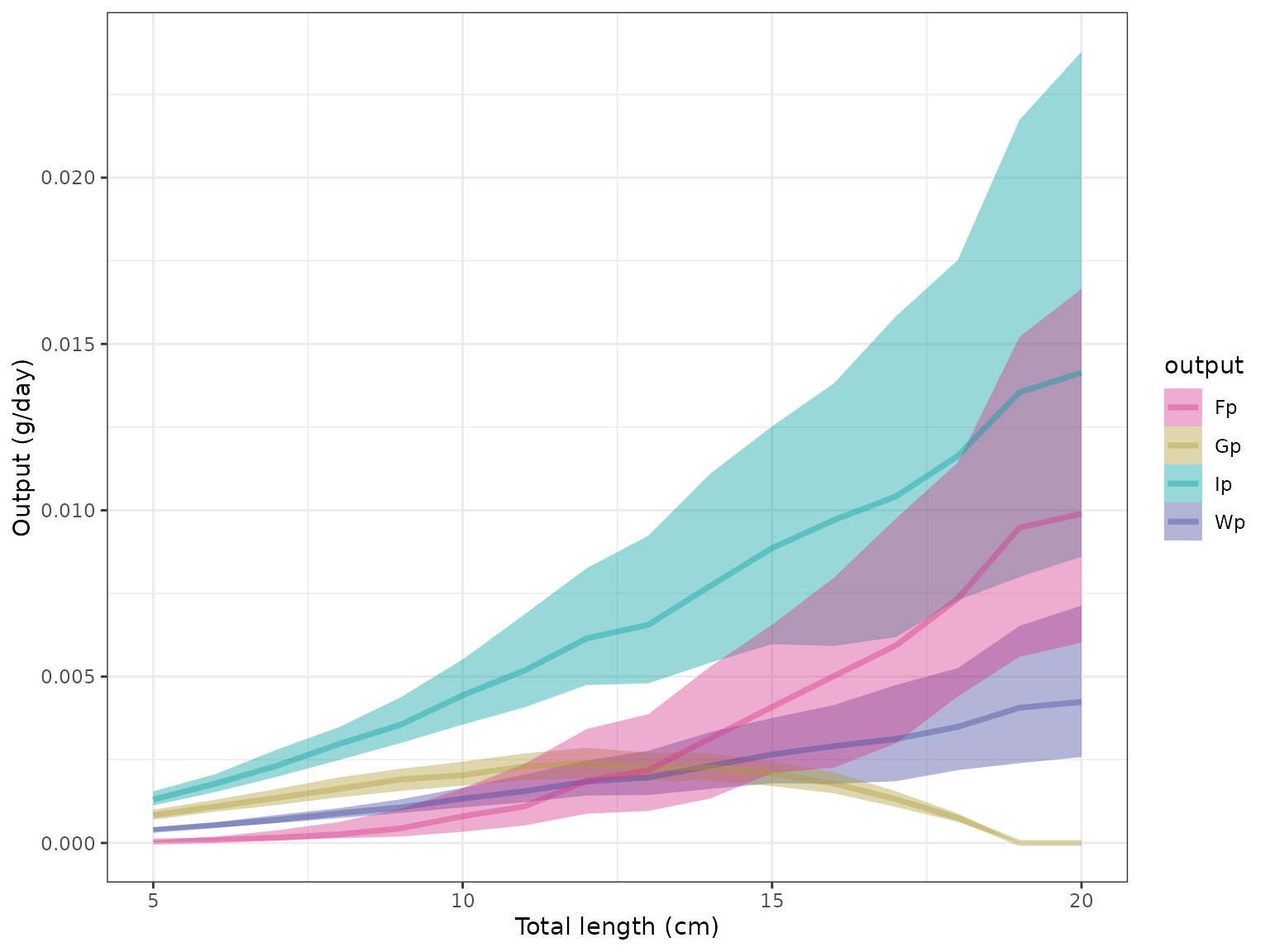
To visualize main outputs of the model, fishflux
contains a plotting function. The function limitation()
returns the proportion of iterations of the model simulation that had
limitation of C, N and P respectively. The function
plot_cnp() plots the predicted output of the model.
## limitation
limitation(model)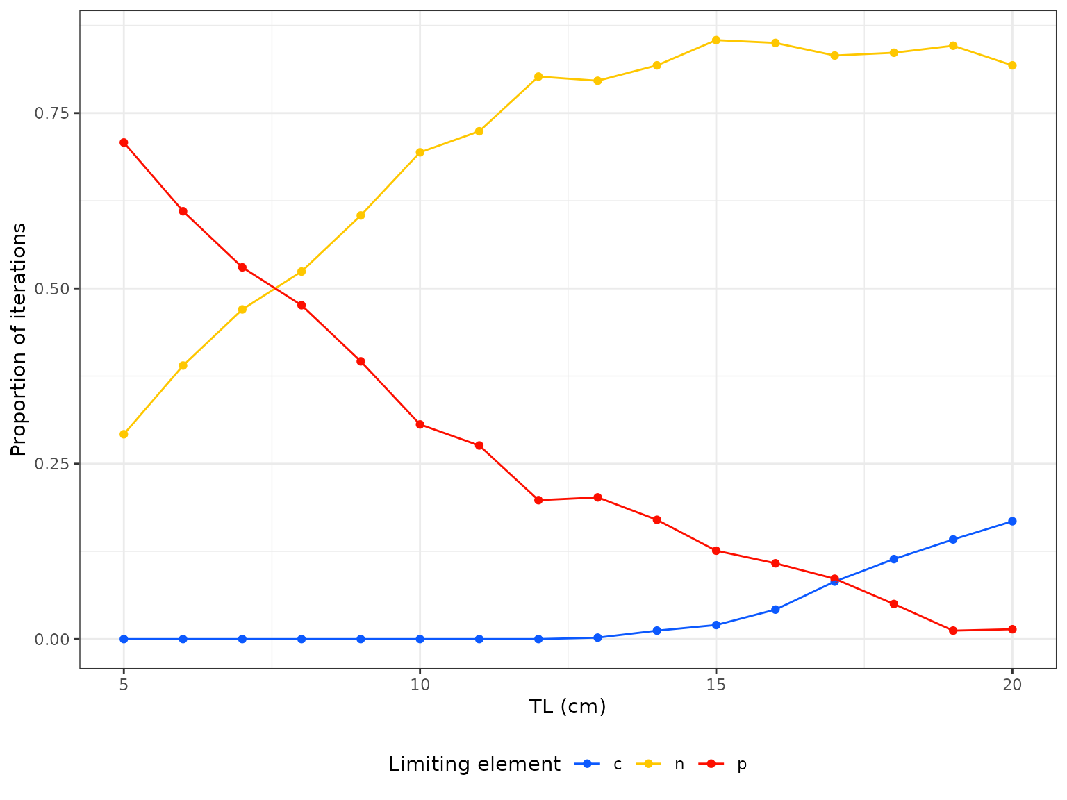
#>    tl nutrient prop_lim
#> 1   5        c    0.000
#> 2   6        c    0.000
#> 3   7        c    0.000
#> 4   8        c    0.000
#> 5   9        c    0.000
#> 6  10        c    0.000
#> 7  11        c    0.000
#> 8  12        c    0.000
#> 9  13        c    0.002
#> 10 14        c    0.012
#> 11 15        c    0.020
#> 12 16        c    0.042
#> 13 17        c    0.082
#> 14 18        c    0.114
#> 15 19        c    0.142
#> 16 20        c    0.168
#> 17  5        n    0.292
#> 18  6        n    0.390
#> 19  7        n    0.470
#> 20  8        n    0.524
#> 21  9        n    0.604
#> 22 10        n    0.694
#> 23 11        n    0.724
#> 24 12        n    0.802
#> 25 13        n    0.796
#> 26 14        n    0.818
#> 27 15        n    0.854
#> 28 16        n    0.850
#> 29 17        n    0.832
#> 30 18        n    0.836
#> 31 19        n    0.846
#> 32 20        n    0.818
#> 33  5        p    0.708
#> 34  6        p    0.610
#> 35  7        p    0.530
#> 36  8        p    0.476
#> 37  9        p    0.396
#> 38 10        p    0.306
#> 39 11        p    0.276
#> 40 12        p    0.198
#> 41 13        p    0.202
#> 42 14        p    0.170
#> 43 15        p    0.126
#> 44 16        p    0.108
#> 45 17        p    0.086
#> 46 18        p    0.050
#> 47 19        p    0.012
#> 48 20        p    0.014
## Plot one variable:
plot_cnp(model,  y = "Fp", x = "tl", probs = c(0.5, 0.8, 0.95))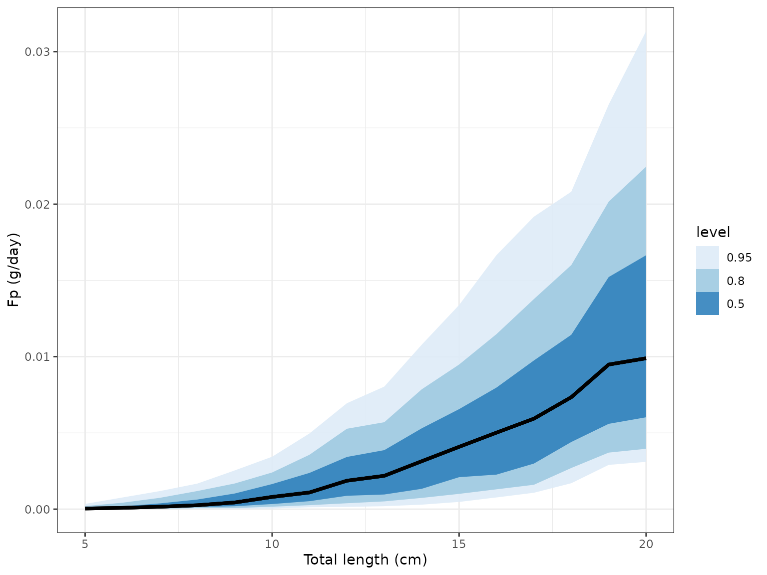
Sensitivity
The function sensitivity() looks at how the distribution
of the input variables affects the uncertainty of the model predictions.
Basically, the model is run for each input parameter, while keeping all
the others fixed. The output of the function gives a matrix of the width
of the 95% CI for all model predictions (columns), depending on the
input variables (rows). The input parameters and output variables of
interest can be specified by arguments “par” and “out” respectively.
sensitivity(TL = 10, param = list(k_sd = 0.2, Dn_sd = 0.2, Dc_sd = 0.1),
            par = c("k_sd","Dn_sd","Dc_sd"),
            out = c("Ic", "In", "Ip", "Gc"))
#> Warning in cnp_mcmc(TL, param, iter, params_st, cor, ...): not inputting
#> certain parameters may give wrong results
#> Warning in cnp_mcmc(TL, param, iter, params_st, cor, ...): adding standard
#> values for ac_m
#> Warning in cnp_mcmc(TL, param, iter, params_st, cor, ...): adding standard
#> values for an_m
#> Warning in cnp_mcmc(TL, param, iter, params_st, cor, ...): adding standard
#> values for ap_m
#> Warning in cnp_mcmc(TL, param, iter, params_st, cor, ...): adding standard
#> values for Dc_m
#> Warning in cnp_mcmc(TL, param, iter, params_st, cor, ...): adding standard
#> values for Dn_m
#> Warning in cnp_mcmc(TL, param, iter, params_st, cor, ...): adding standard
#> values for Dp_m
#> Warning in cnp_mcmc(TL, param, iter, params_st, cor, ...): adding standard
#> values for linf_m
#> Warning in cnp_mcmc(TL, param, iter, params_st, cor, ...): adding standard
#> values for k_m
#> Warning in cnp_mcmc(TL, param, iter, params_st, cor, ...): adding standard
#> values for t0_m
#> Warning in cnp_mcmc(TL, param, iter, params_st, cor, ...): adding standard
#> values for theta_m
#> Warning in cnp_mcmc(TL, param, iter, params_st, cor, ...): adding standard
#> values for r_m
#> Warning in cnp_mcmc(TL, param, iter, params_st, cor, ...): adding standard
#> values for h_m
#> Warning in cnp_mcmc(TL, param, iter, params_st, cor, ...): adding standard
#> values for lwa_m
#> Warning in cnp_mcmc(TL, param, iter, params_st, cor, ...): adding standard
#> values for lwb_m
#> Warning in cnp_mcmc(TL, param, iter, params_st, cor, ...): adding standard
#> values for mdw_m
#> Warning in cnp_mcmc(TL, param, iter, params_st, cor, ...): adding standard
#> values for v_m
#> Warning in cnp_mcmc(TL, param, iter, params_st, cor, ...): adding standard
#> values for F0nz_m
#> Warning in cnp_mcmc(TL, param, iter, params_st, cor, ...): adding standard
#> values for F0pz_m
#> Warning in cnp_mcmc(TL, param, iter, params_st, cor, ...): adding standard
#> values for Qc_m
#> Warning in cnp_mcmc(TL, param, iter, params_st, cor, ...): adding standard
#> values for Qn_m
#> Warning in cnp_mcmc(TL, param, iter, params_st, cor, ...): adding standard
#> values for Qp_m
#> Warning in cnp_mcmc(TL, param, iter, params_st, cor, ...): adding standard
#> values for alpha_m
#> Warning in cnp_mcmc(TL, param, iter, params_st, cor, ...): adding standard
#> values for f0_m
#> Warning in cnp_mcmc(TL, param, iter, params_st, cor, ...): adding standard
#> values for lt_sd
#> Warning in cnp_mcmc(TL, param, iter, params_st, cor, ...): adding standard
#> values for ac_sd
#> Warning in cnp_mcmc(TL, param, iter, params_st, cor, ...): adding standard
#> values for an_sd
#> Warning in cnp_mcmc(TL, param, iter, params_st, cor, ...): adding standard
#> values for ap_sd
#> Warning in cnp_mcmc(TL, param, iter, params_st, cor, ...): adding standard
#> values for Dp_sd
#> Warning in cnp_mcmc(TL, param, iter, params_st, cor, ...): adding standard
#> values for linf_sd
#> Warning in cnp_mcmc(TL, param, iter, params_st, cor, ...): adding standard
#> values for t0_sd
#> Warning in cnp_mcmc(TL, param, iter, params_st, cor, ...): adding standard
#> values for theta_sd
#> Warning in cnp_mcmc(TL, param, iter, params_st, cor, ...): adding standard
#> values for r_sd
#> Warning in cnp_mcmc(TL, param, iter, params_st, cor, ...): adding standard
#> values for h_sd
#> Warning in cnp_mcmc(TL, param, iter, params_st, cor, ...): adding standard
#> values for lwa_sd
#> Warning in cnp_mcmc(TL, param, iter, params_st, cor, ...): adding standard
#> values for lwb_sd
#> Warning in cnp_mcmc(TL, param, iter, params_st, cor, ...): adding standard
#> values for mdw_sd
#> Warning in cnp_mcmc(TL, param, iter, params_st, cor, ...): adding standard
#> values for v_sd
#> Warning in cnp_mcmc(TL, param, iter, params_st, cor, ...): adding standard
#> values for F0nz_sd
#> Warning in cnp_mcmc(TL, param, iter, params_st, cor, ...): adding standard
#> values for F0pz_sd
#> Warning in cnp_mcmc(TL, param, iter, params_st, cor, ...): adding standard
#> values for Qc_sd
#> Warning in cnp_mcmc(TL, param, iter, params_st, cor, ...): adding standard
#> values for Qn_sd
#> Warning in cnp_mcmc(TL, param, iter, params_st, cor, ...): adding standard
#> values for Qp_sd
#> Warning in cnp_mcmc(TL, param, iter, params_st, cor, ...): adding standard
#> values for alpha_sd
#> Warning in cnp_mcmc(TL, param, iter, params_st, cor, ...): adding standard
#> values for f0_sd
#>
#> SAMPLING FOR MODEL 'cnpmodelmcmc' NOW (CHAIN 1).
#> Chain 1: Iteration:   1 / 1000 [  0%]  (Sampling)
#> Chain 1: Iteration: 100 / 1000 [ 10%]  (Sampling)
#> Chain 1: Iteration: 200 / 1000 [ 20%]  (Sampling)
#> Chain 1: Iteration: 300 / 1000 [ 30%]  (Sampling)
#> Chain 1: Iteration: 400 / 1000 [ 40%]  (Sampling)
#> Chain 1: Iteration: 500 / 1000 [ 50%]  (Sampling)
#> Chain 1: Iteration: 600 / 1000 [ 60%]  (Sampling)
#> Chain 1: Iteration: 700 / 1000 [ 70%]  (Sampling)
#> Chain 1: Iteration: 800 / 1000 [ 80%]  (Sampling)
#> Chain 1: Iteration: 900 / 1000 [ 90%]  (Sampling)
#> Chain 1: Iteration: 1000 / 1000 [100%]  (Sampling)
#> Chain 1:
#> Chain 1:  Elapsed Time: 0 seconds (Warm-up)
#> Chain 1:                0.005 seconds (Sampling)
#> Chain 1:                0.005 seconds (Total)
#> Chain 1: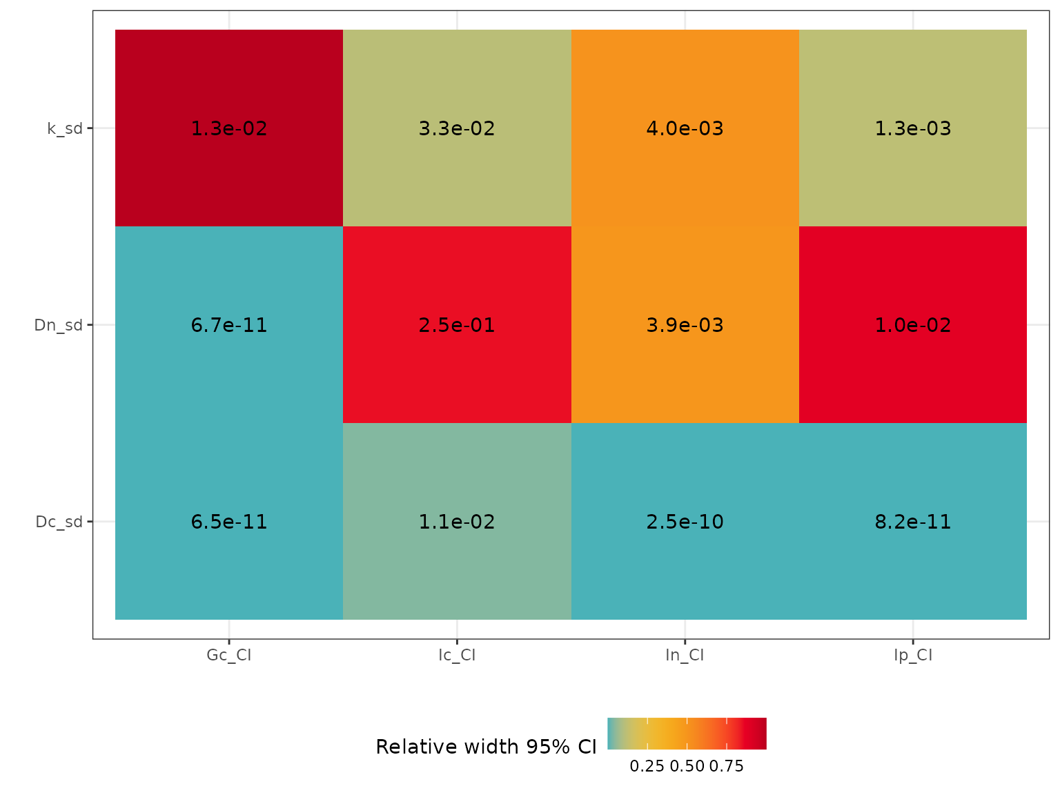
#>            Ic_CI        In_CI        Ip_CI        Gc_CI
#> k_sd  0.03296944 3.956333e-03 1.318778e-03 1.266026e-02
#> Dn_sd 0.24950299 3.859819e-03 9.980120e-03 6.731756e-11
#> Dc_sd 0.01112390 2.464069e-10 8.188419e-11 6.544082e-11
More information
For more information on the theoretical framework of the model, see
Schiettekatte et al. (2020) ( paper ). Every
function of fishflux has a help page with more
documentation. In the case of errors, bugs or discomfort, you are
invited to raise an issue on GitHub.
fishflux is always in development and we are happy to take
your comments or suggestions into consideration.