Somatic growth of fishes is a fundamental trait that determines essential ecosystem services such as food provision and nutrient cycling. Growth rate information can be derived through age estimation based on the analysis of sagittal otoliths. While fitting growth models on size-at-age data is the most frequently employed approach to deriving growth parameters, this method requires a high number of individuals. An alternative approach based on back-calculation can provide approximations to individual-level growth trajectories. fishgrowbot provides functions to perform the back-calculation in a Bayesian framework. Further, the package provides a Bayesian framework to fit the von Bertalanffy growth model to the back-calculated lengths in a hierarchical structure. Finally, fishgrowbot provides functions to visualize the results. In this vignette, we provide an introduction to fishgrowbot through a case study. For more theoretical background of the methodology, see Morat et al. (2020)
First things first: we need to load some packages.
library(fishgrowbot)
library(dplyr)
#>
#> Attaching package: 'dplyr'
#> The following objects are masked from 'package:stats':
#>
#>     filter, lag
#> The following objects are masked from 'package:base':
#>
#>     intersect, setdiff, setequal, union
To introduce the functionalities of fishgrowbot, we look at an example for Epinephelus merra. The function bcalc() returns both a dataframe with the back-calculated lengths and their uncertainty and the model object for more details on the fit of the bc stan model.
The input data should contain:
+ id: Unique fish id per individual.
+ radi: Measurements of otolith growth rings (in mm).
+ agei: Age estimation of fish.
+ lencap: Length at capture (in mm).
+ radcap: Radius of otolith at capture (in mm).
+ l0p: Length of fish at hatching (in mm).
# get data
em <- filter(coral_reef_fishes_data, species == "Epinephelus merra",
             location == "Moorea")
# back-calculation
bc <- bcalc(data = em)
#>
#> SAMPLING FOR MODEL 'stan_bcalc' NOW (CHAIN 1).
#> Chain 1:
#> Chain 1: Gradient evaluation took 4.7e-05 seconds
#> Chain 1: 1000 transitions using 10 leapfrog steps per transition would take 0.47 seconds.
#> Chain 1: Adjust your expectations accordingly!
#> Chain 1:
#> Chain 1:
#> Chain 1: Iteration:    1 / 2000 [  0%]  (Warmup)
#> Chain 1: Iteration:  200 / 2000 [ 10%]  (Warmup)
#> Chain 1: Iteration:  400 / 2000 [ 20%]  (Warmup)
#> Chain 1: Iteration:  600 / 2000 [ 30%]  (Warmup)
#> Chain 1: Iteration:  800 / 2000 [ 40%]  (Warmup)
#> Chain 1: Iteration: 1000 / 2000 [ 50%]  (Warmup)
#> Chain 1: Iteration: 1001 / 2000 [ 50%]  (Sampling)
#> Chain 1: Iteration: 1200 / 2000 [ 60%]  (Sampling)
#> Chain 1: Iteration: 1400 / 2000 [ 70%]  (Sampling)
#> Chain 1: Iteration: 1600 / 2000 [ 80%]  (Sampling)
#> Chain 1: Iteration: 1800 / 2000 [ 90%]  (Sampling)
#> Chain 1: Iteration: 2000 / 2000 [100%]  (Sampling)
#> Chain 1:
#> Chain 1:  Elapsed Time: 0.671087 seconds (Warm-up)
#> Chain 1:                0.191103 seconds (Sampling)
#> Chain 1:                0.86219 seconds (Total)
#> Chain 1:
#>
#> SAMPLING FOR MODEL 'stan_bcalc' NOW (CHAIN 2).
#> Chain 2:
#> Chain 2: Gradient evaluation took 2.7e-05 seconds
#> Chain 2: 1000 transitions using 10 leapfrog steps per transition would take 0.27 seconds.
#> Chain 2: Adjust your expectations accordingly!
#> Chain 2:
#> Chain 2:
#> Chain 2: Iteration:    1 / 2000 [  0%]  (Warmup)
#> Chain 2: Iteration:  200 / 2000 [ 10%]  (Warmup)
#> Chain 2: Iteration:  400 / 2000 [ 20%]  (Warmup)
#> Chain 2: Iteration:  600 / 2000 [ 30%]  (Warmup)
#> Chain 2: Iteration:  800 / 2000 [ 40%]  (Warmup)
#> Chain 2: Iteration: 1000 / 2000 [ 50%]  (Warmup)
#> Chain 2: Iteration: 1001 / 2000 [ 50%]  (Sampling)
#> Chain 2: Iteration: 1200 / 2000 [ 60%]  (Sampling)
#> Chain 2: Iteration: 1400 / 2000 [ 70%]  (Sampling)
#> Chain 2: Iteration: 1600 / 2000 [ 80%]  (Sampling)
#> Chain 2: Iteration: 1800 / 2000 [ 90%]  (Sampling)
#> Chain 2: Iteration: 2000 / 2000 [100%]  (Sampling)
#> Chain 2:
#> Chain 2:  Elapsed Time: 0.708654 seconds (Warm-up)
#> Chain 2:                0.209596 seconds (Sampling)
#> Chain 2:                0.91825 seconds (Total)
#> Chain 2:
#>
#> SAMPLING FOR MODEL 'stan_bcalc' NOW (CHAIN 3).
#> Chain 3:
#> Chain 3: Gradient evaluation took 2.9e-05 seconds
#> Chain 3: 1000 transitions using 10 leapfrog steps per transition would take 0.29 seconds.
#> Chain 3: Adjust your expectations accordingly!
#> Chain 3:
#> Chain 3:
#> Chain 3: Iteration:    1 / 2000 [  0%]  (Warmup)
#> Chain 3: Iteration:  200 / 2000 [ 10%]  (Warmup)
#> Chain 3: Iteration:  400 / 2000 [ 20%]  (Warmup)
#> Chain 3: Iteration:  600 / 2000 [ 30%]  (Warmup)
#> Chain 3: Iteration:  800 / 2000 [ 40%]  (Warmup)
#> Chain 3: Iteration: 1000 / 2000 [ 50%]  (Warmup)
#> Chain 3: Iteration: 1001 / 2000 [ 50%]  (Sampling)
#> Chain 3: Iteration: 1200 / 2000 [ 60%]  (Sampling)
#> Chain 3: Iteration: 1400 / 2000 [ 70%]  (Sampling)
#> Chain 3: Iteration: 1600 / 2000 [ 80%]  (Sampling)
#> Chain 3: Iteration: 1800 / 2000 [ 90%]  (Sampling)
#> Chain 3: Iteration: 2000 / 2000 [100%]  (Sampling)
#> Chain 3:
#> Chain 3:  Elapsed Time: 0.635907 seconds (Warm-up)
#> Chain 3:                0.201078 seconds (Sampling)
#> Chain 3:                0.836985 seconds (Total)
#> Chain 3:
#>
#> SAMPLING FOR MODEL 'stan_bcalc' NOW (CHAIN 4).
#> Chain 4:
#> Chain 4: Gradient evaluation took 2.7e-05 seconds
#> Chain 4: 1000 transitions using 10 leapfrog steps per transition would take 0.27 seconds.
#> Chain 4: Adjust your expectations accordingly!
#> Chain 4:
#> Chain 4:
#> Chain 4: Iteration:    1 / 2000 [  0%]  (Warmup)
#> Chain 4: Iteration:  200 / 2000 [ 10%]  (Warmup)
#> Chain 4: Iteration:  400 / 2000 [ 20%]  (Warmup)
#> Chain 4: Iteration:  600 / 2000 [ 30%]  (Warmup)
#> Chain 4: Iteration:  800 / 2000 [ 40%]  (Warmup)
#> Chain 4: Iteration: 1000 / 2000 [ 50%]  (Warmup)
#> Chain 4: Iteration: 1001 / 2000 [ 50%]  (Sampling)
#> Chain 4: Iteration: 1200 / 2000 [ 60%]  (Sampling)
#> Chain 4: Iteration: 1400 / 2000 [ 70%]  (Sampling)
#> Chain 4: Iteration: 1600 / 2000 [ 80%]  (Sampling)
#> Chain 4: Iteration: 1800 / 2000 [ 90%]  (Sampling)
#> Chain 4: Iteration: 2000 / 2000 [100%]  (Sampling)
#> Chain 4:
#> Chain 4:  Elapsed Time: 0.674606 seconds (Warm-up)
#> Chain 4:                0.226985 seconds (Sampling)
#> Chain 4:                0.901591 seconds (Total)
#> Chain 4:
head(bc$lengths)
#>                   id age      l_m         l_sd     l_lb     l_ub
#> 1 EP_ME_MO_03_16_001   0   1.5000 1.075803e-15   1.5000   1.5000
#> 2 EP_ME_MO_03_16_001   1 154.2769 5.916885e+00 142.4640 165.7040
#> 3 EP_ME_MO_03_16_001   2 178.3752 4.688731e+00 168.9472 187.3399
#> 4 EP_ME_MO_03_16_001   3 192.1466 3.843450e+00 184.3903 199.4565
#> 5 EP_ME_MO_03_16_001   4 205.6511 2.921718e+00 199.7355 211.1807
#> 6 EP_ME_MO_03_16_001   5 217.7558 2.022035e+00 213.6506 221.5667
The function bcplot helps visualize the back calculation. Some examples:
bcplot(bc$lengths)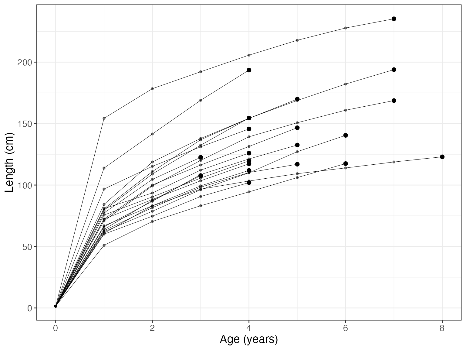
bcplot(bc$lengths, colorid = TRUE)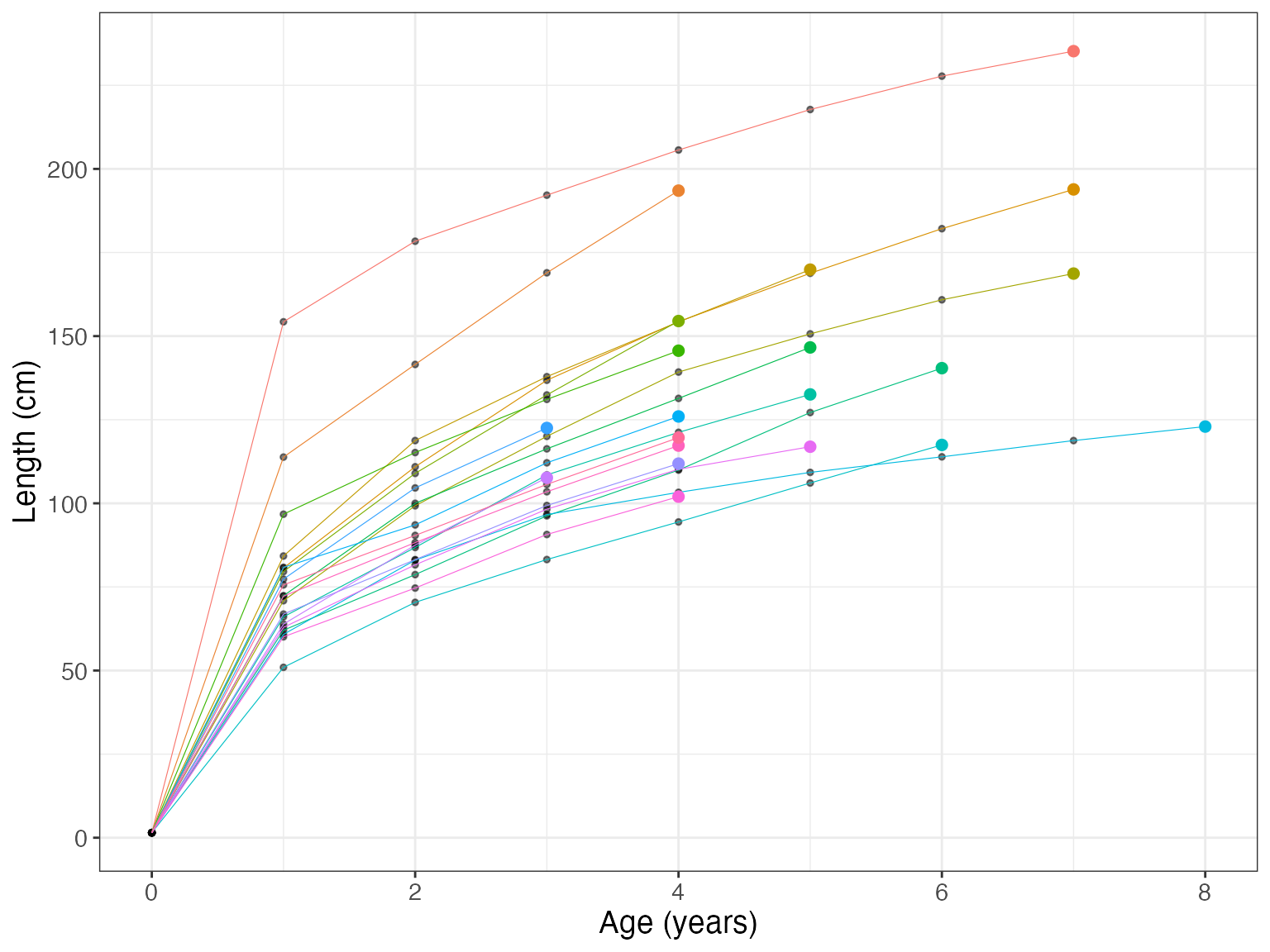
bcplot(bc$lengths, colorid = TRUE, facet = TRUE, error = TRUE)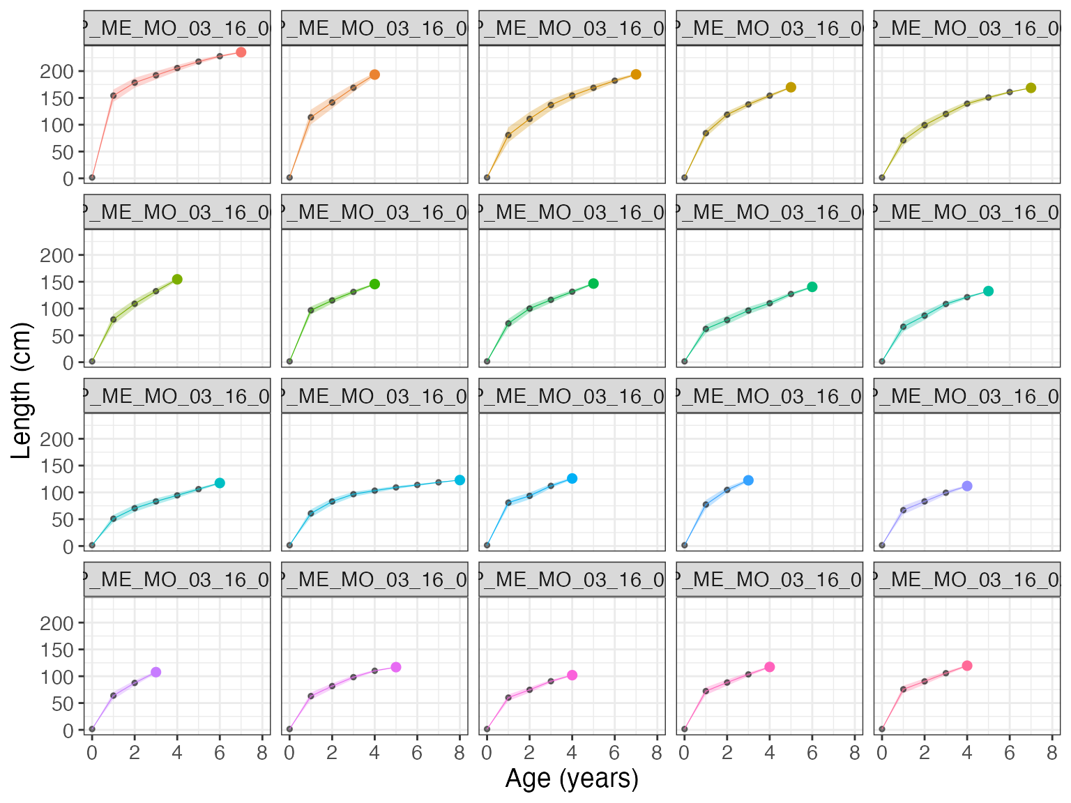
Then, we can fit the hierarchical von Bertalanffy growth model that allows for the estimation of multiple parameters. Importantly, length measures should be given in cm.
# fit growth model
growthmodel <- growthreg(length = bc$lengths$l_m / 10, age =  bc$lengths$age,
                         id =  bc$lengths$id, lmax = 32, linf_m = 28,
                         linf_sd = 5, l0_m = 0.15, l0_sd = 0.015, iter = 4000,
                         open_progress = FALSE, plot = FALSE)
#>
#> SAMPLING FOR MODEL 'vonbert' NOW (CHAIN 1).
#> Chain 1:
#> Chain 1: Gradient evaluation took 9.2e-05 seconds
#> Chain 1: 1000 transitions using 10 leapfrog steps per transition would take 0.92 seconds.
#> Chain 1: Adjust your expectations accordingly!
#> Chain 1:
#> Chain 1:
#> Chain 1: Iteration:    1 / 4000 [  0%]  (Warmup)
#> Chain 1: Iteration:  400 / 4000 [ 10%]  (Warmup)
#> Chain 1: Iteration:  800 / 4000 [ 20%]  (Warmup)
#> Chain 1: Iteration: 1200 / 4000 [ 30%]  (Warmup)
#> Chain 1: Iteration: 1600 / 4000 [ 40%]  (Warmup)
#> Chain 1: Iteration: 2000 / 4000 [ 50%]  (Warmup)
#> Chain 1: Iteration: 2001 / 4000 [ 50%]  (Sampling)
#> Chain 1: Iteration: 2400 / 4000 [ 60%]  (Sampling)
#> Chain 1: Iteration: 2800 / 4000 [ 70%]  (Sampling)
#> Chain 1: Iteration: 3200 / 4000 [ 80%]  (Sampling)
#> Chain 1: Iteration: 3600 / 4000 [ 90%]  (Sampling)
#> Chain 1: Iteration: 4000 / 4000 [100%]  (Sampling)
#> Chain 1:
#> Chain 1:  Elapsed Time: 9.83133 seconds (Warm-up)
#> Chain 1:                11.9846 seconds (Sampling)
#> Chain 1:                21.8159 seconds (Total)
#> Chain 1:
#>
#> SAMPLING FOR MODEL 'vonbert' NOW (CHAIN 2).
#> Chain 2:
#> Chain 2: Gradient evaluation took 6.4e-05 seconds
#> Chain 2: 1000 transitions using 10 leapfrog steps per transition would take 0.64 seconds.
#> Chain 2: Adjust your expectations accordingly!
#> Chain 2:
#> Chain 2:
#> Chain 2: Iteration:    1 / 4000 [  0%]  (Warmup)
#> Chain 2: Iteration:  400 / 4000 [ 10%]  (Warmup)
#> Chain 2: Iteration:  800 / 4000 [ 20%]  (Warmup)
#> Chain 2: Iteration: 1200 / 4000 [ 30%]  (Warmup)
#> Chain 2: Iteration: 1600 / 4000 [ 40%]  (Warmup)
#> Chain 2: Iteration: 2000 / 4000 [ 50%]  (Warmup)
#> Chain 2: Iteration: 2001 / 4000 [ 50%]  (Sampling)
#> Chain 2: Iteration: 2400 / 4000 [ 60%]  (Sampling)
#> Chain 2: Iteration: 2800 / 4000 [ 70%]  (Sampling)
#> Chain 2: Iteration: 3200 / 4000 [ 80%]  (Sampling)
#> Chain 2: Iteration: 3600 / 4000 [ 90%]  (Sampling)
#> Chain 2: Iteration: 4000 / 4000 [100%]  (Sampling)
#> Chain 2:
#> Chain 2:  Elapsed Time: 8.12538 seconds (Warm-up)
#> Chain 2:                9.78997 seconds (Sampling)
#> Chain 2:                17.9154 seconds (Total)
#> Chain 2:
#>
#> SAMPLING FOR MODEL 'vonbert' NOW (CHAIN 3).
#> Chain 3:
#> Chain 3: Gradient evaluation took 6.4e-05 seconds
#> Chain 3: 1000 transitions using 10 leapfrog steps per transition would take 0.64 seconds.
#> Chain 3: Adjust your expectations accordingly!
#> Chain 3:
#> Chain 3:
#> Chain 3: Iteration:    1 / 4000 [  0%]  (Warmup)
#> Chain 3: Iteration:  400 / 4000 [ 10%]  (Warmup)
#> Chain 3: Iteration:  800 / 4000 [ 20%]  (Warmup)
#> Chain 3: Iteration: 1200 / 4000 [ 30%]  (Warmup)
#> Chain 3: Iteration: 1600 / 4000 [ 40%]  (Warmup)
#> Chain 3: Iteration: 2000 / 4000 [ 50%]  (Warmup)
#> Chain 3: Iteration: 2001 / 4000 [ 50%]  (Sampling)
#> Chain 3: Iteration: 2400 / 4000 [ 60%]  (Sampling)
#> Chain 3: Iteration: 2800 / 4000 [ 70%]  (Sampling)
#> Chain 3: Iteration: 3200 / 4000 [ 80%]  (Sampling)
#> Chain 3: Iteration: 3600 / 4000 [ 90%]  (Sampling)
#> Chain 3: Iteration: 4000 / 4000 [100%]  (Sampling)
#> Chain 3:
#> Chain 3:  Elapsed Time: 8.21418 seconds (Warm-up)
#> Chain 3:                10.7795 seconds (Sampling)
#> Chain 3:                18.9937 seconds (Total)
#> Chain 3:
#>
#> SAMPLING FOR MODEL 'vonbert' NOW (CHAIN 4).
#> Chain 4:
#> Chain 4: Gradient evaluation took 6.5e-05 seconds
#> Chain 4: 1000 transitions using 10 leapfrog steps per transition would take 0.65 seconds.
#> Chain 4: Adjust your expectations accordingly!
#> Chain 4:
#> Chain 4:
#> Chain 4: Iteration:    1 / 4000 [  0%]  (Warmup)
#> Chain 4: Iteration:  400 / 4000 [ 10%]  (Warmup)
#> Chain 4: Iteration:  800 / 4000 [ 20%]  (Warmup)
#> Chain 4: Iteration: 1200 / 4000 [ 30%]  (Warmup)
#> Chain 4: Iteration: 1600 / 4000 [ 40%]  (Warmup)
#> Chain 4: Iteration: 2000 / 4000 [ 50%]  (Warmup)
#> Chain 4: Iteration: 2001 / 4000 [ 50%]  (Sampling)
#> Chain 4: Iteration: 2400 / 4000 [ 60%]  (Sampling)
#> Chain 4: Iteration: 2800 / 4000 [ 70%]  (Sampling)
#> Chain 4: Iteration: 3200 / 4000 [ 80%]  (Sampling)
#> Chain 4: Iteration: 3600 / 4000 [ 90%]  (Sampling)
#> Chain 4: Iteration: 4000 / 4000 [100%]  (Sampling)
#> Chain 4:
#> Chain 4:  Elapsed Time: 8.04411 seconds (Warm-up)
#> Chain 4:                10.0493 seconds (Sampling)
#> Chain 4:                18.0934 seconds (Total)
#> Chain 4:
# summary growth parameters
growthmodel$summary
#>             mean      se_mean         sd        2.5%         25%        50%
#> k     0.64388071 0.0011928339 0.05339357  0.54716951  0.60680606  0.6413700
#> linf 14.98680283 0.0342464087 1.00943121 13.08767706 14.30894104 14.9484589
#> l0    0.41902598 0.0037563714 0.23514567 -0.04919666  0.25917832  0.4239523
#> t0   -0.04514989 0.0004188101 0.02639038 -0.09810503 -0.06272757 -0.0447222
#> kmax  0.39675488 0.0007768033 0.04099917  0.32369332  0.36745898  0.3945958
#>              75%       97.5%
#> k     0.67724213  0.75641030
#> linf 15.63495883 17.04643201
#> l0    0.57813663  0.86700492
#> t0   -0.02677341  0.00471082
#> kmax  0.42321755  0.48392668
We can use existing packages rstan and bayesplot to make diagnostic plots.
library(rstan)
#> Loading required package: StanHeaders
#> Loading required package: ggplot2
#> rstan (Version 2.21.2, GitRev: 2e1f913d3ca3)
#> For execution on a local, multicore CPU with excess RAM we recommend calling
#> options(mc.cores = parallel::detectCores()).
#> To avoid recompilation of unchanged Stan programs, we recommend calling
#> rstan_options(auto_write = TRUE)
library(bayesplot)
#> This is bayesplot version 1.8.0
#> - Online documentation and vignettes at mc-stan.org/bayesplot
#> - bayesplot theme set to bayesplot::theme_default()
#>    * Does _not_ affect other ggplot2 plots
#>    * See ?bayesplot_theme_set for details on theme setting
# Posterior predictive check
yrep <- extract(growthmodel$stanfit, "y_rep")$y_rep
ppc_dens_overlay(y = bc$lengths$l_m / 10, yrep = yrep[1:100,])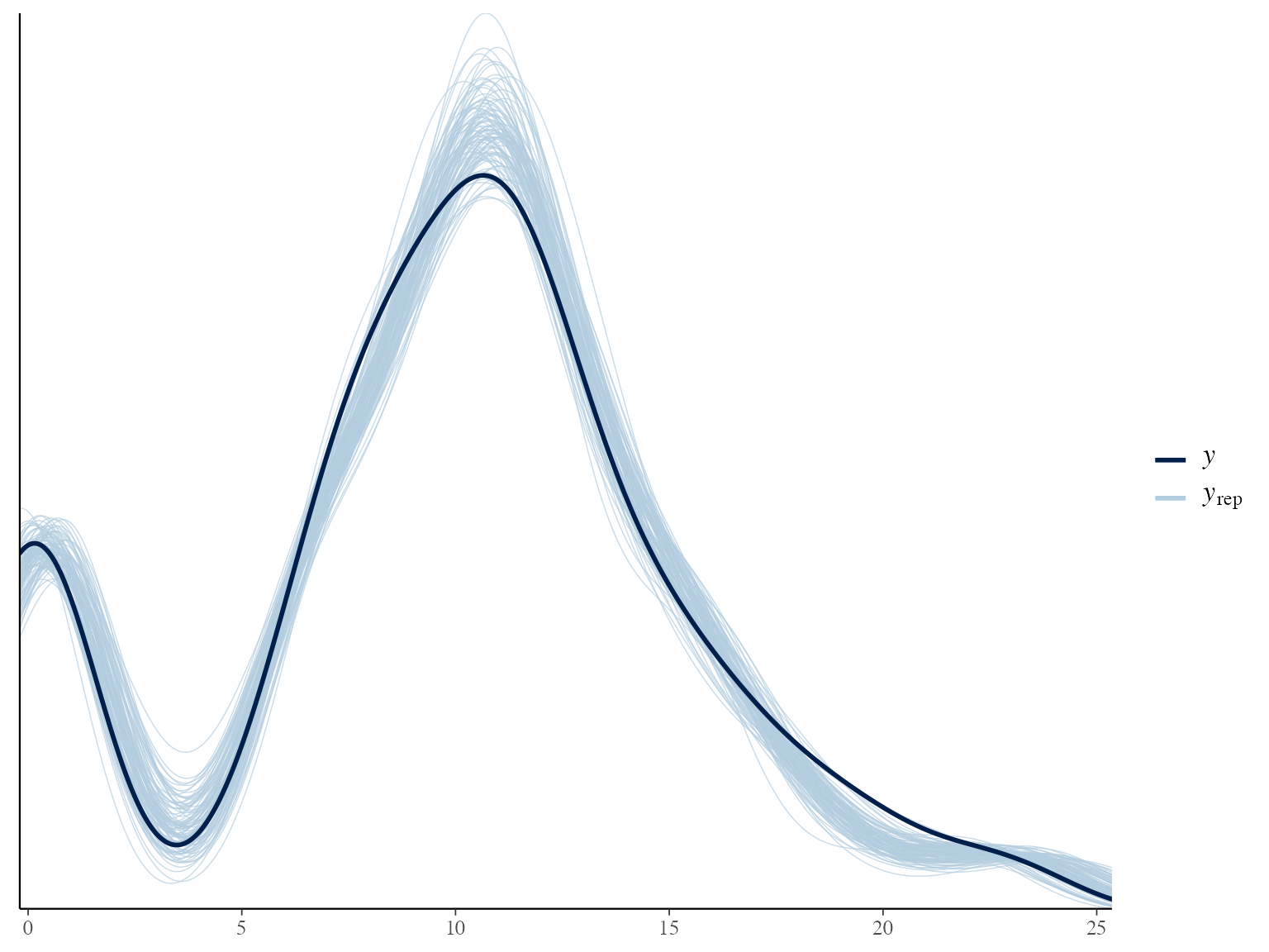
#trace plots
posterior <- extract(growthmodel$stanfit, permuted = FALSE)

p <- mcmc_trace(posterior,  pars = c("linf", "k"),
                facet_args = list(nrow = 2, labeller = label_parsed))
p + facet_text(size = 15)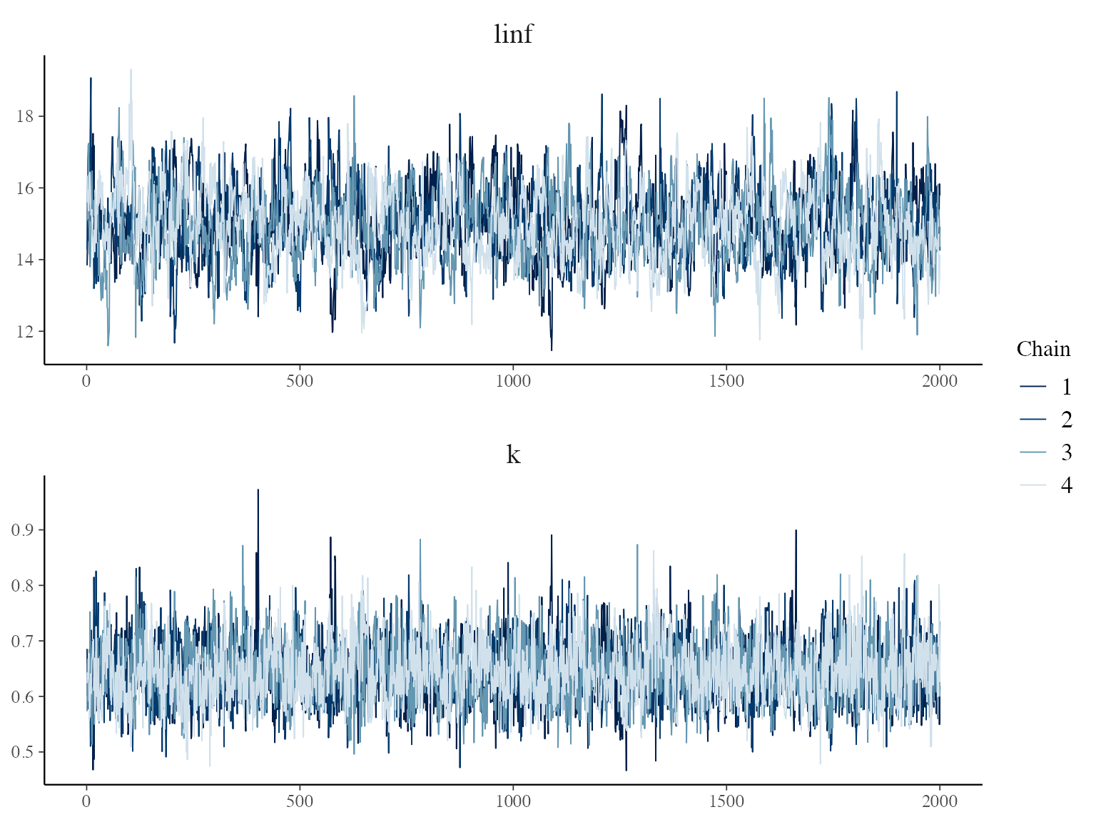
Now we can visualize the fit with the function gmplot().
gmplot(growthmodel)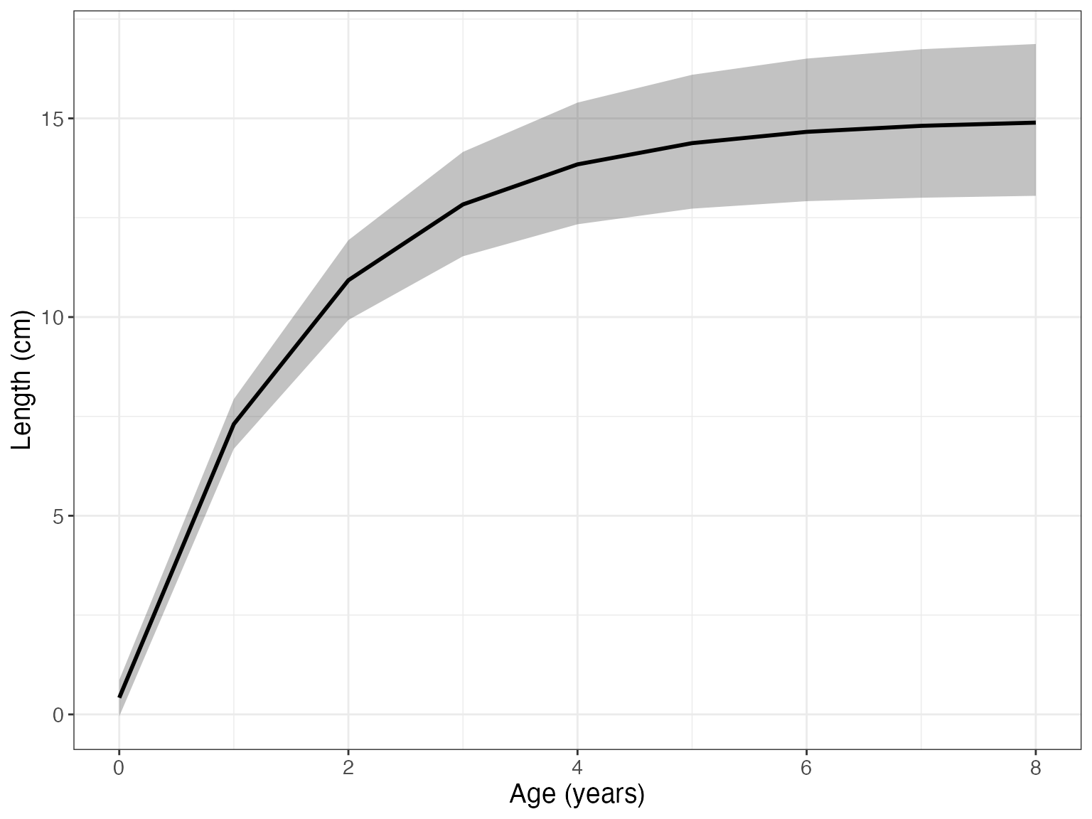
Setting id = TRUE, we can see the individual growth curves.
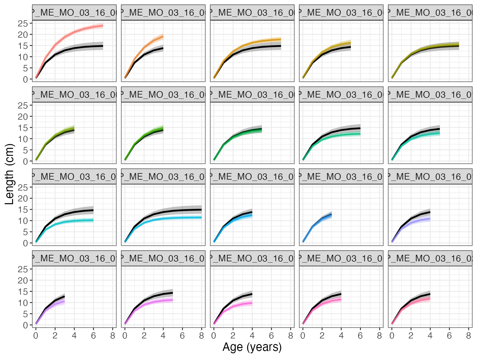
gmplot(growthmodel, id = TRUE)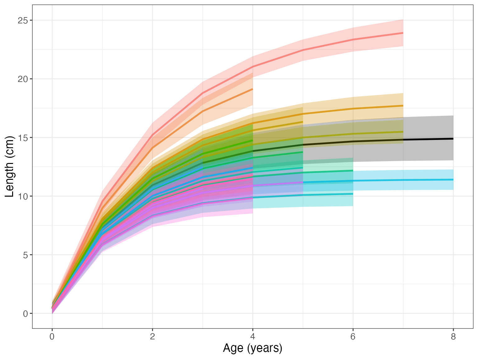
If there are many individuals, the id graph can quickly get crowded. Set facet = TRUE to have a subplot per individual.
gmplot(growthmodel, id = TRUE, facet = TRUE)